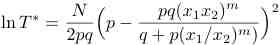
where T* is the number of trials and m is the moment of the distribution that we wish to estimate. How does the estimate of T* compare with the results you observe in the simulation?
Introduction
Examples of random multiplicative processes include the distributions of incomes, rainfall, and fragment sizes in rock crushing processes. Consider the latter for which we begin with a rock of size w. We strike the rock with a hammer and generate two fragments whose sizes are pw and qw, where q = 1 - p. In the next step the possible sizes of the fragments are p2w, pqw, qpw, and q2w. What is the distribution of the fragments after N blows of the hammer?
To answer this question, consider a binary sequence in which the numbers x1 and x2 appear independently with probabilities p and q respectively. If there are N elements in the product Π, we can ask what is <Π>, the mean value of Π? To compute <Π>, we define P(n) as the probability that the product of N independent factors of x1 and x2 has the value x1n x2N-n. This probability is given by the number of sequences where x1 appears n times multiplied by the probability of choosing a specific sequence with x1 appearing n times:
P(n) = N!/(n! (N - n)!) pn qN-n.
The mean value of the product is given by
<Π> = Σn=0 P(n) x1nx2N-n = (px1 + qx2)N.
The most probable event is one in which the product contains Np factors of x1 and Nq factors of x2. Hence, the most probable value of the product is
Πmp = (x1px2q)N.
Problems
References
Java Classes
Updated 28 December 2009.