Direct Monte Carlo Computation of the Partition Function

Introduction

The Wang-Landau algorithm computes the density of states directly by doing a biased random walk. The idea is to make changes at random, but to sample energies that are more probable less often so that all states are sampled equally. An algorithm due to Zhang and Ma allows us to compute the partition function directly using an algorithm similar to the Wang-Landau algorithm. The modified algorithm uses two types of trial moves: a standard Metropolis Monte Carlo move such as a flip of a spin which changes the energy at fixed temperature, and a move to change the temperature at fixed energy. The idea is that the random temperature changes will range over low and high temperatures so that rare energy states can be sampled more efficiently. We will discuss the algorithm in the context of the two-dimensional Ising model.

Algorithm

The algorithm can be summarized by the following steps:

1. Set up an array of temperatures T. In the simulation we chose values of T from T = 0.1 to T = 8 with 218 temperature bins; the bin width was reduced for temperatures near the critical value. Set the estimate of the logarithm of the partition function in each bin to zero. We use the logarithm because the partition function grows very rapidly with energy.
2. Choose an initial value of the modification parameter f as in the Wang-Landau algorithm. We take f₀ = e ≅ 2.71. The number of Monte Carlo moves per spin for a given f is chosen to be (100)/√(ln f).
3. Choose the probability p of a trial temperature change. For a 32 × 32 lattice we chose p = 0.01. Otherwise make a standard Monte Carlo step.
4. Begin with a random starting configuration and an initial temperature T_i.
5. Compute the total energy of the current state.
6. If an energy move is chosen, flip a spin and accept the trial change with the usual Metropolis probability at the current temperature.
7. If a temperature move is chosen, randomly choose a temperature T_j. Accept the new temperature with the probability

   ,

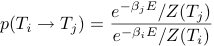   where β = 1/T is the inverse temperature. If the new temperature is accepted, then T_i → T_j.
8. Regardless of which type of change was chosen, update the partition function by

   ln Z(T_i) → ln Z(T_i) + ln f.

9. After the fixed number of Monte Carlo moves chosen in step 2, reduce f as in the Wang-Landau algorithm; that is, f → √(f).
10. Stop the simulation when ln f < 10^-9.

    The algorithm yields the log of the partition function up to a constant. We will display values of ln Z relative to its value at the lowest temperature T = 0.1.

    The acceptance rule in step 7 is consistent with detailed balance with a probability distribution given by the Boltzmann distribution. If the current estimate of the partition function for a particular temperature is too low, the algorithm will favor moves toward that temperature, thus eventually approaching the correct value for the partition function. Sometimes the simulation does not accurately compute the low temperature values for Z because not enough time was spent there. One way to tell is to check if ln Z is a monotonically increasing function of temperature. Thus, it is important to do several independent runs.

Problems

Note that if the display delay is set to the default value, there will be a delay when you stop the program. However, the program will run much faster. The optimum value of display delay depends on the speed of your computer.

1. Run the simulation for a small system (2 × 2) and compare your results with the exact value for Z, which you can calculate analytically. Describe the qualitative temperature dependence of the partition function.
2. Run the simulation for a larger system. How does the partition function for the larger system compare to that of the smaller one? Explore various size lattices. Are the estimated results for the partition function always a monotonic increasing function of the temperature as they should be?
3. Describe the qualitative nature of the changing spin configurations.
4. Increase the probability of choosing a temperature move. Are your results different? If so, why?
5. Why do we set the probability for choosing a temperature move so much less than the probability of choosing an energy move?

References

• J. Kim, J. E. Straub, and T. Keyes, “Statistical temperature Monte Carlo and molecular dynamics algorithms,” Phys. Rev. Lett. 97, 050601-1–4 (2006).
• F. Wang and D. P. Landau, “Efficient, multiple-range random walk algorithm to calculate the density of states,” Phys. Rev. Lett. 86, 2050–2053 (2001), and “Determining the density of states for classical statistical models: A random walk algorithm to produce a flat histogram,” Phys. Rev. E 64, 056101-1–16 (2001).
• Cheng Zhang and Jianpeng Ma, “Simulation via direct computation of partition functions,” Phys. Rev. E 76, 036708-1–5 (2007).

Java Classes

• PartFuncCalc
• PartFuncCalcApp

Modified 28 December 2009.