The binomial distribution

Introduction

The binomial distribution is the result of a Bernoulli process. In such a process each trial has only two outcomes and the result of each trial is independent of all previous trials. Examples of a Bernoulli process are the flips of a coin, the random walk of a drunken sailor in one dimension, and a system of noninteracting magnetic moments with spin 1/2.

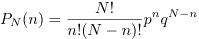
    To be specific we consider a system of N noninteracting magnetic moments (spins). Each spin has a probability p of being up and a probability q = 1 - p of pointing down. What is the probability that n spins are up? The answer is given by the binomial distribution:

P_N(n) is the probability that n spins are up out of N spins.

The Program

Because P_N(n) involves factorials, it is not easy to evaluate P_N for large N. To handle N > 20, the program uses Stirling's approximation:

Questions

1. Calculate the form of P_N(n) for N = 3 and arbitrary p by enumerating the eight possible microstates (configurations) and compare your result to the results of the program. (You can obtain the numerical results by selecting Data Table under the Views menu.)
2. Plot P_N(n) for increasing values of N with p = 1/2. What is the qualitative dependence of the width of P_N(n) on N? Also compare the relative heights of the maximum of P_N(n).
3. The program plots P_N(n) for various values of N in the same size window. Does the width of the distribution appear to become larger or smaller as N is increased?
4. Compare the plots of P_N(n) versus n to the plots of P_N(n) versus n/<n>. What can you conclude about the N-dependence of the width of P_N?
5. Plot ln P_N(n) versus n for N = 16. (Choose Log Axes under the Views menu.) Describe the behavior of ln P_N(n). Can it be fitted to a parabola?

Java Classes

• BinomialApp

Updated 4 March 2009.